Category: Projects

  • How do you count a million milk crates?

    We were losing hundreds of thousands of milk crates a year. At $4 a piece, it was half a million dollars. Conventional wisdom was that the majority of the loss was stores using them for storage, or people taking them home for furniture or their garage, but the volume we were seeing had nothing to do with people wanting cheap shelving.

    A hidden supply chain

    Milk crates are made out of high-density polyethylene, and HDPE is a commodity whose price tracks crude oil. A single crate weighs about three pounds, and a recycler will pay 14 to 28 cents a pound for ground plastic, depending on the market. Each crate brings 50 to 80 cents in scrap value, free money if you don’t pay for the crate itself.

    The crews work at night, driving behind grocery stores and bakeries and loading empty crates off the dock. From there, the crates go to a rented warehouse with an industrial grinder inside. Whole crates go in one end. Plastic pellets come out the other. The pellets get bagged and shipped overseas, where they get melted down and turned into pipes and flower pots. Ironically sometimes new crates. A certain percentage of the crates we bought were made out of those stolen in the first place.

    The dairy industry loses 20 to 25 million crates a year this way. $80 to $100 million. One dairy in Downey, lost 424,000 crates in a single year. $1.6 million in replacements, for one plant. The LA County Sheriff’s department had a dedicated unit for it, the Industrial Plastic Theft Task Force, and they recovered $6 million in stolen plastics in one year of raids.

    The Dairy Institute eventually hired a private investigator who ran stings. He’d load up a truck with milk crates and drive around to recyclers offering to sell. Eleven of them bought without question. All eleven got arrested. From there he expanded across Orange, San Diego, and LA counties. Miami ran its own version of the sting and got two dozen arrests plus $1.5 million in stolen crates.

    How do you count what’s missing?

    We knew we were losing crates. We could see it in the replacement costs. But we didn’t know how many were actually being lost, because there were always confounding variables. Were stores holding onto crates in their backrooms, or was it truly missing? If the majority of the crates were still in the network, then it was an operational controls question. If they aren’t, then it’s still an operational controls question, just different levers.

    But we didn’t even know how many were in circulation, which meant we couldn’t measure the loss rate, which meant we couldn’t tell whether anything we tried was working. Not knowing how much was out there was the worst part. Do we plan a large water run or will that cause us to run out of crates and short milk to the stores?

    An email blast would increase the crate return, but was that 10% of the problem or 90%?

    The crates are never all in one place. At any given moment they’re scattered across the creamery, trucks, store back rooms, distribution centers, and a nontrivial number of them are in a warehouse in Commerce getting fed into a grinder. You can’t pause the whole system and count. Ecologists have the same problem with animal populations.

    Capture Recapture

    You can’t count every fish in a lake. But you can estimate it. Capture-recapture. You catch a sample of animals, mark them, release them back into the population, and then wait for them to mix in. When you catch another sample and count how many marked ones show up, you can estimate how big the total population is. Say you marked 100 fish and your second catch of 50 has 5 marked fish in it. That’s 10 percent, so the total population is about 1,000. We did the same thing with milk crates. This solution would let us count crates that were lingering in backrooms and trucks, because the marked crates would mix into the population. Crates that were lost would not be counted.

    We deployed a fixed number of gray crates into the distribution network. Then we waited. Once the system had time to mix, we started counting. Every time a batch of crates came back to the creamery, we recorded how many gray crates were in it.

    The simple Petersen estimator assumes you do your sampling all at once, and our data didn’t work like that. Returns came in over weeks, so we used a beta-binomial model instead. In a beta-binomial setup the true share of colored crates floating around out there is a latent variable, and every returning batch updates it. At the start the estimates come out wide. Then the batches accumulate and the posterior tightens, and you get to watch the uncertainty shrink in real time. It approached an equlibrium.

    For the first time we had a defensible number, the size of the project. How many crates were actually in circulation, how many were gone, and what that was worth in dollars. The annual replacement spend was about $500,000, and from the results we brought in, we estimated that $250,000 of that was organized theft. The retail side had a better staffed loss prevention unit with former detectives that picked up the case from us, once we could show them the scale of the problem.

    What I think about milk crates

    Milk crate and plastic reusable container loss is still significant, but decreasing. The last project I worked on at the company when I left was on a different type of theft. The tools for combatting it have gotten more sophisticated, but the underpinning needing to have numbers that square with reality hasn’t. A recurring theme on this blog is accurate measurement, and for me, the milk crates episode encapsulates that. Not knowing if on the other side of the wall you have 200,000 crates or 0 is a legitimately terrifying feeling. Vibes aren’t good enough.

  • Making Tempeh: An Unreasonably Thorough Approach

    Making Tempeh: An Unreasonably Thorough Approach

    I have had so much trouble making tempeh. Crumbly, inconsistent results, batch after batch. And the troubleshooting guides online? Useless. Every single one boils down to the same set of contradictions:

    • You cooked the beans too much
    • You cooked the beans too little
    • You dried the beans too much
    • You dried the beans too little
    • You incubated too hot
    • You incubated too cold
    • You packed too tight
    • You packed too loose
    • You split the beans too much
    • You split the beans too little

    Right. So that narrows it down to everything. I decided the only way forward was to go clinical, document every step, measure every variable, and remove every excuse. If this batch failed, I’d know exactly how and why.

    Cracking the Beans

    Most instructions say to soak the beans and then scrub the hulls off by hand, squeezing each one between your fingers. I skipped that entirely. It’s a waste of water and time when you can just pre-crack them.

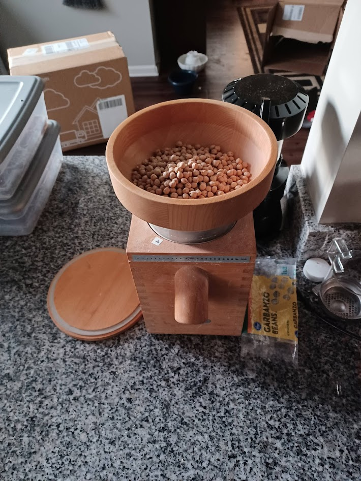
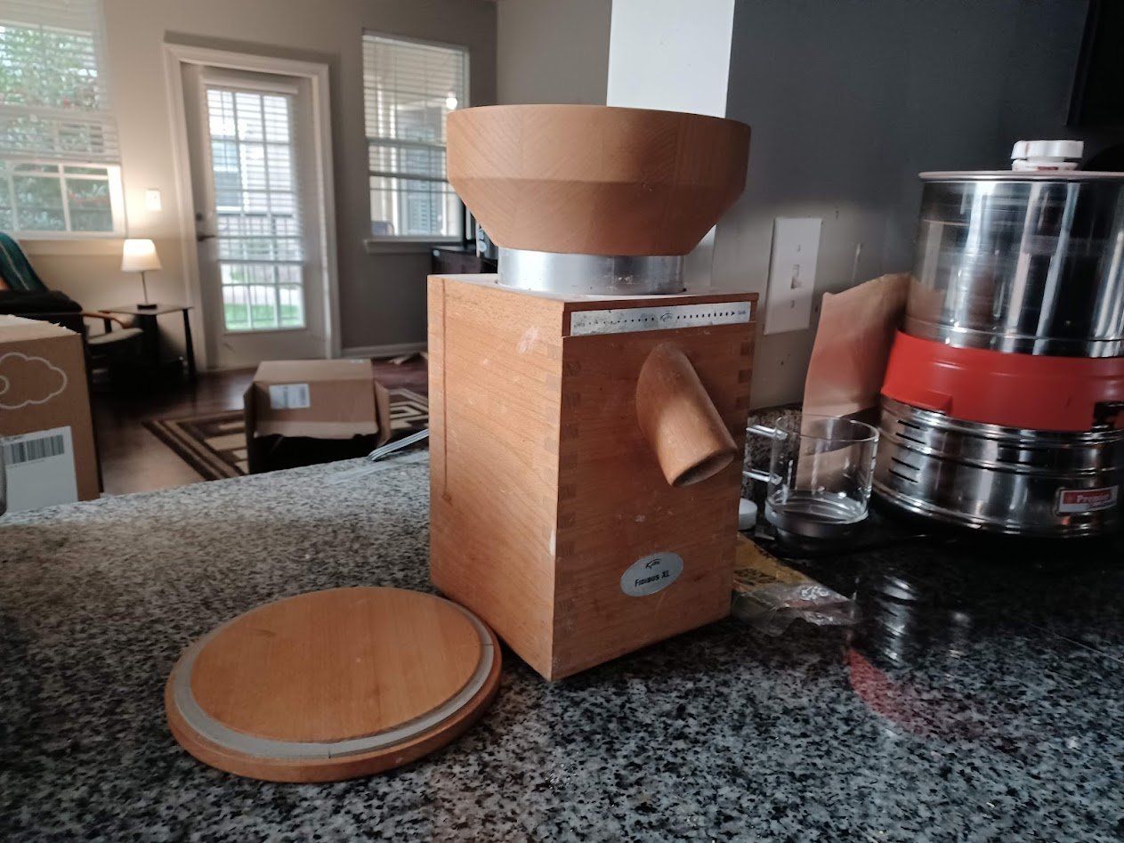
    KoMo Fidibus XL grain mill on granite countertop
    My KoMo Fidibus XL. I’ve had this mill for over a decade and it has paid for itself many times over.
    Soybeans loaded in the grain mill hopper
    Soybeans loaded and ready to crack.

    I widened the grinding wheels and ran a few test passes until I found a setting that splits the beans in half without creating too much dust. When you crack them this way, the hulls tend to fall right off.

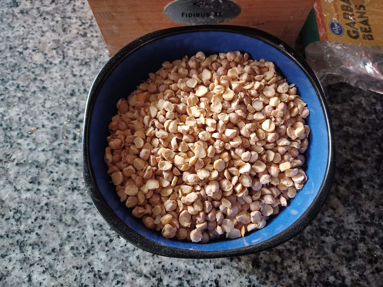
    A note: this post mixes photos from two batches, one garbanzo, one soybean. The process is the same for both.

    Cracked garbanzo beans in a blue bowl
    Cracked and dehulled in about two minutes.
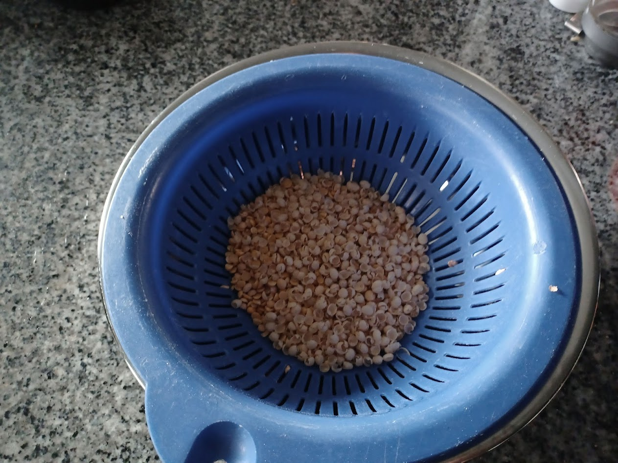
    Bean hulls and dust in a blue colander
    Running the cracked beans through a colander to sift out the dust.

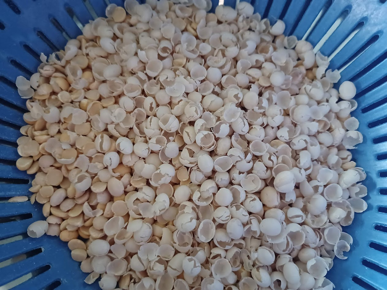
    I shook the colander a few times and the empty hulls floated to the top. A quick pass with a hair dryer, one I keep in the kitchen specifically for cooking, cleared them off in a couple of passes.

    Clean split soybean halves in a blue colander
    Clean splits. Hulls removed, minimal dust.

    I boiled the beans until they reached the consistency of a boiled peanut, maybe a lima bean. Soft enough to eat, firm enough to hold shape. I didn’t photograph this step because it’s just boiling beans.

    The Bags

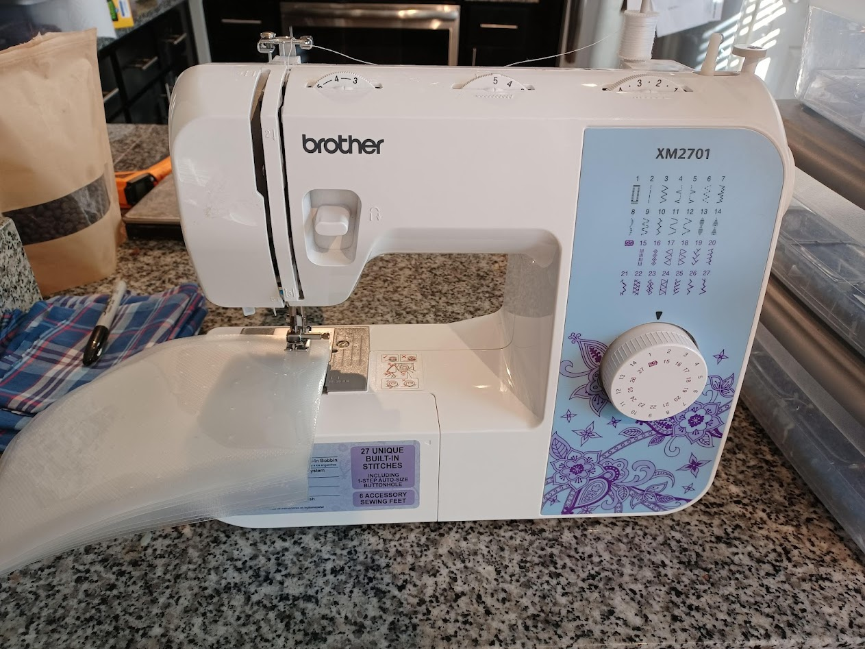
    Brother XM2701 sewing machine
    The sewing machine. Another piece of equipment that’s earned its counter space.

    I read a paper that described optimal tempeh incubation using bags with holes punched by a number 7 needle, spaced half an inch apart, on 1.5mm polyethylene. Here’s what I actually used a size 12 sewing needle at one-inch intervals on a 3mm polyethylene bag. Size 12 is thicker than size 7.

    Drying and Inoculation

    This is the step I suspect most guides don’t emphasize enough, and where most batches quietly go wrong.

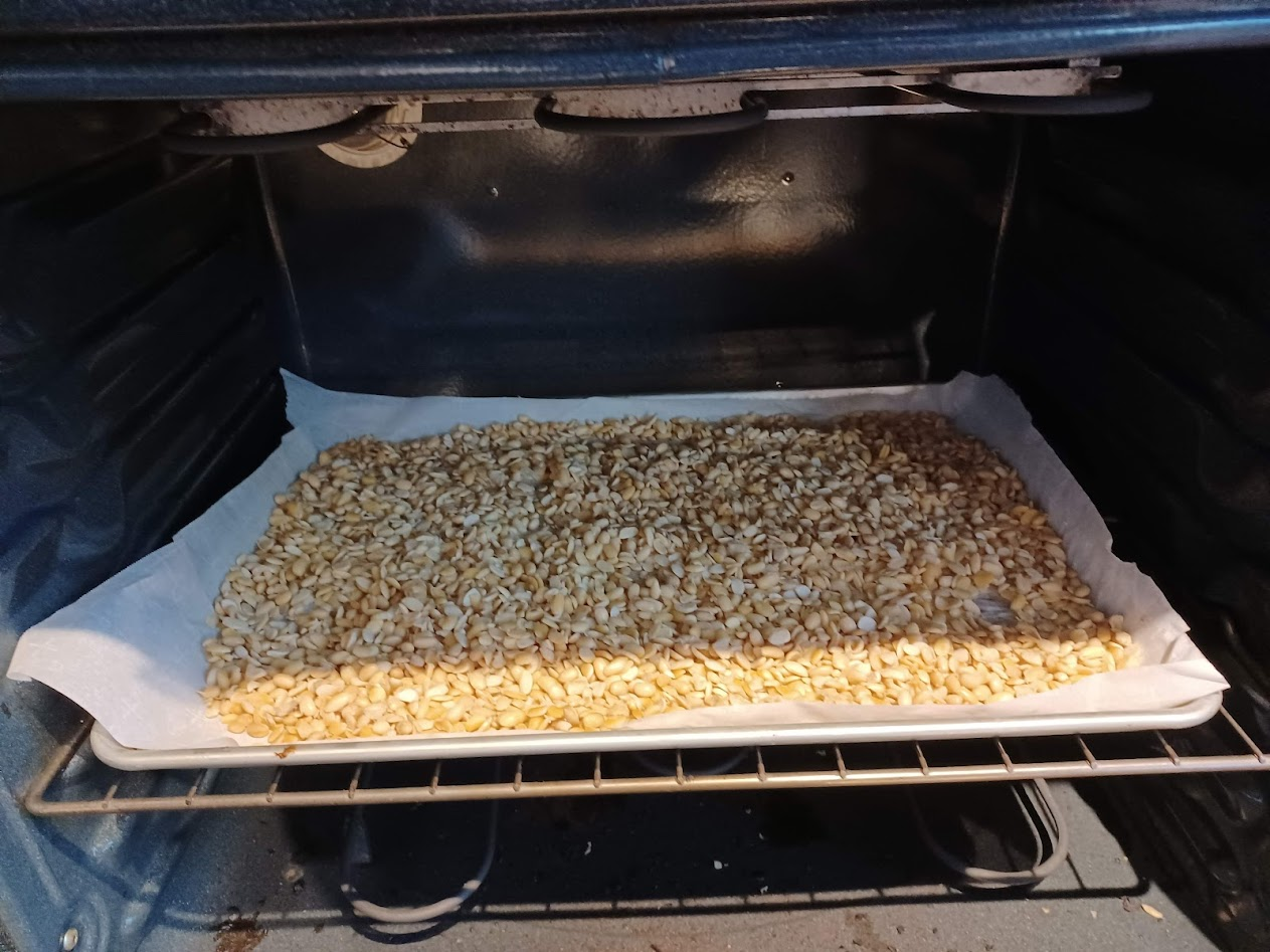
    Beans drying on a parchment-lined baking sheet in the oven
    Drying in the oven at 170°F, stirring every few minutes.

    I set my oven to 170°F and stirred every few minutes until the beans were dry. Actually dry, not “they look dry.” Dry as in my hand doesn’t get wet when I grab a handful. I raised my fist to my face and told each bean it would become tempeh or die.

    Once the surface moisture was gone, I added a few tablespoons of distilled white vinegar and let that evaporate too. The vinegar lowers the pH enough to give the Rhizopus a head start over competing bacteria.

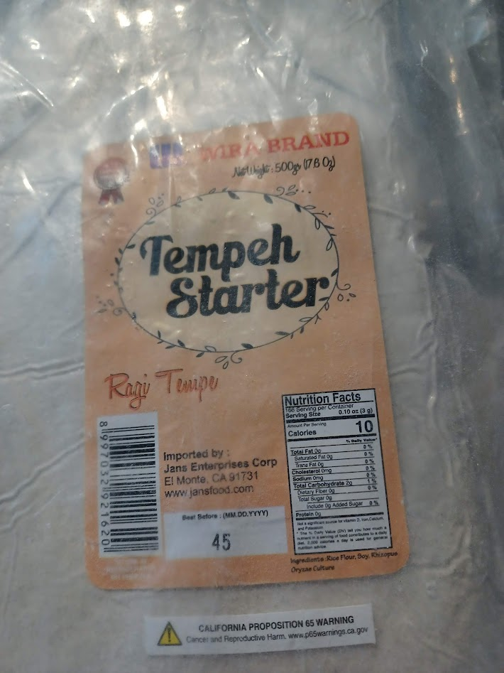
    Tempeh starter packet labeled Ragi Tempe
    The tempeh starter (Rhizopus oligosporus). Kept in my freezer until needed.

    Mixed the starter into the cooled, dry beans. Packed them into the perforated bags, pressed flat to about an inch thick, sealed them up.

    Incubation

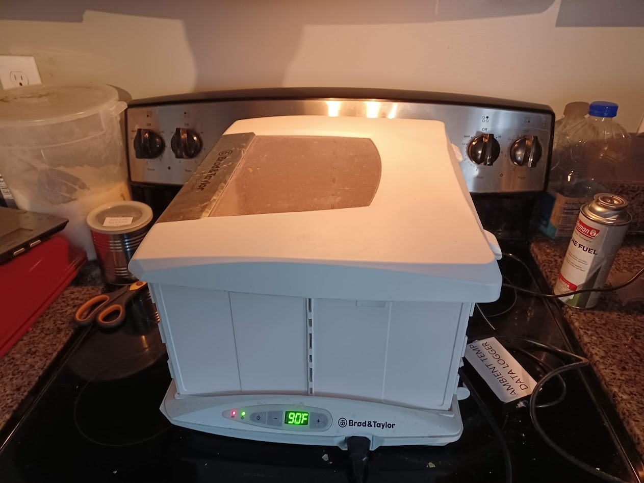
    Brod and Taylor folding proofer displaying 90 degrees
    The Brod & Taylor folding proofer, set to 90°F. Designed for bread, but it holds temperature precisely enough for fermentation work.

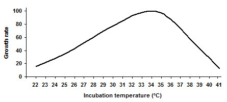
    At this point I hadn’t confirmed the optimal incubation range. A quick search turned up this:

    Growth rate vs incubation temperature chart for Rhizopus
    Rhizopus growth rate peaks around 30–35°C (86–95°F) and drops sharply above 37°C. Source: tempeh.info

    I adjusted to 86°F and loaded the bags.

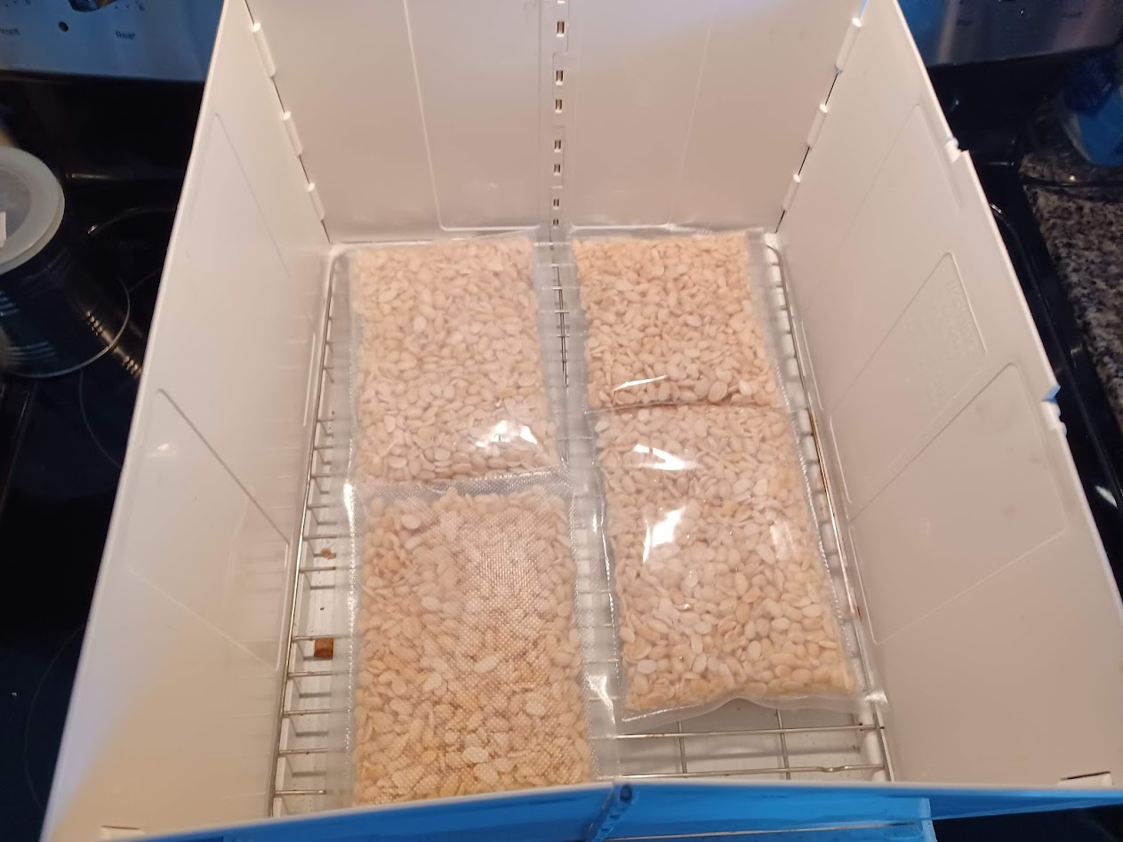
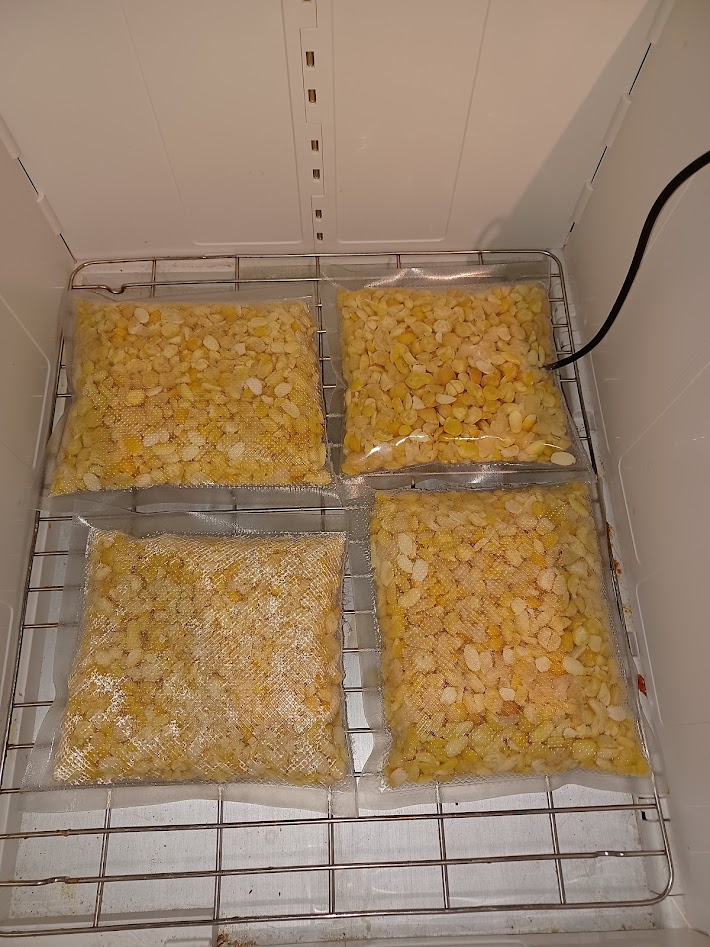
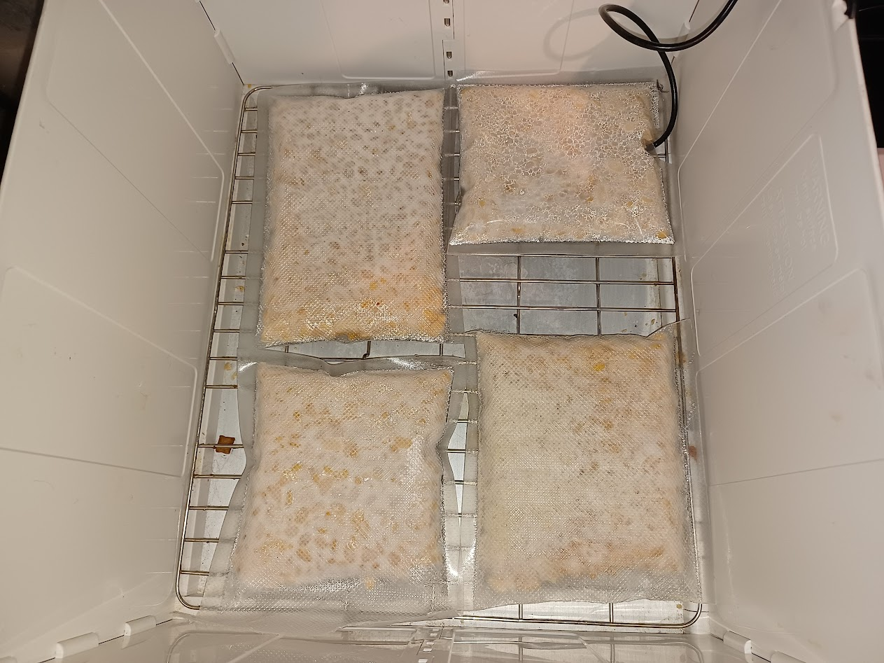
    Four bags of inoculated beans in the incubator
    Four bags loaded, day zero. No visible growth.

    Over-Engineering the Monitoring

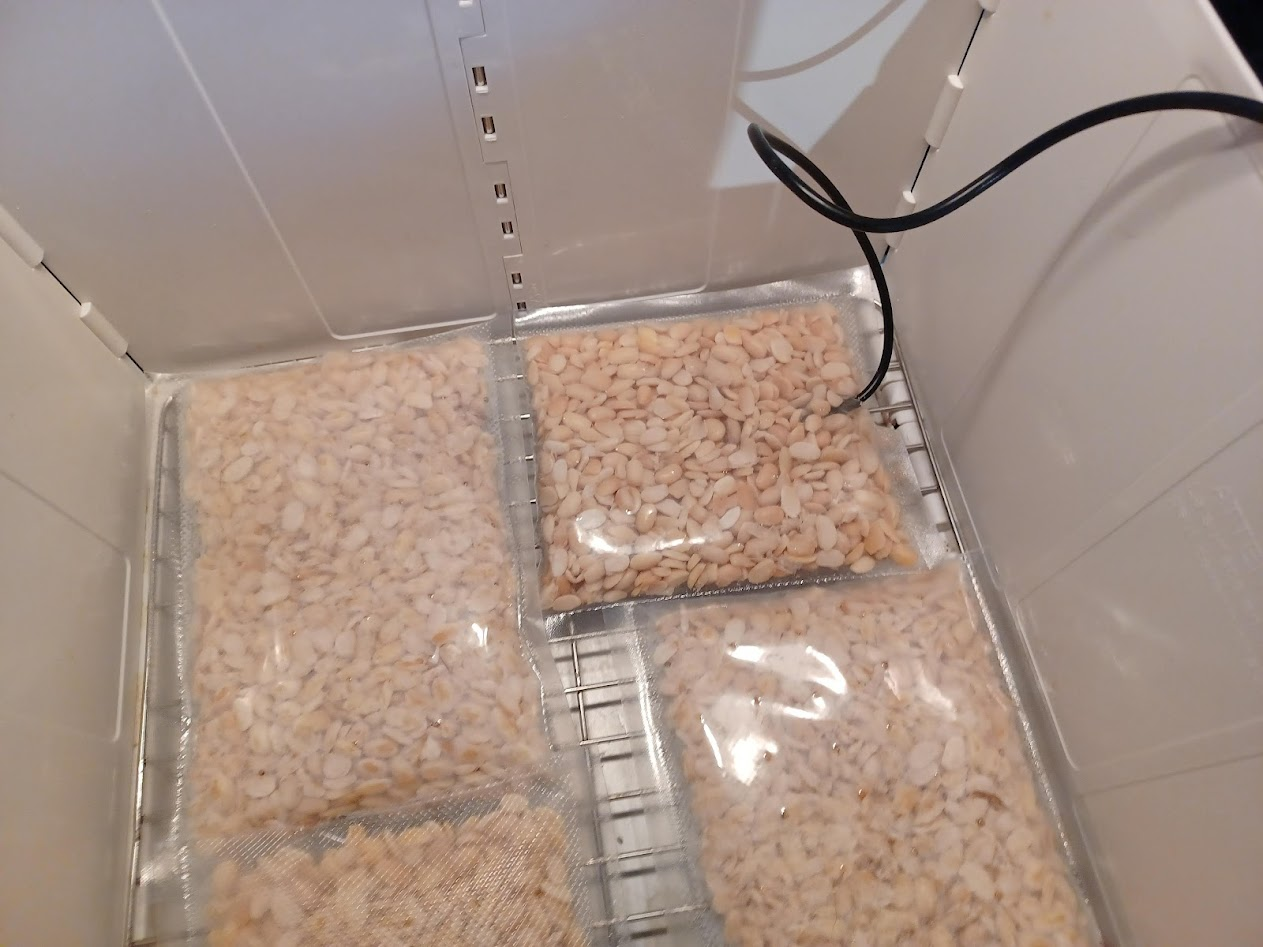
    I wanted the actual temperature inside the bean cake, not just the ambient air reading from the incubator’s display. So I ran a probe thermometer directly into one of the bags.

    Temperature probe cable running into the incubator
    Temperature probe running into the bean cake.

    Then I built a data logger.

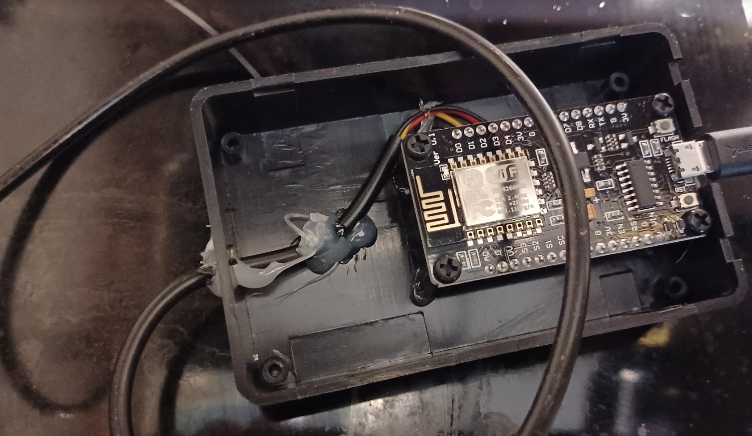
    An ESP8266 microcontroller, programmed with Arduino to read the temperature sensor and transmit data over WiFi at three-second intervals.

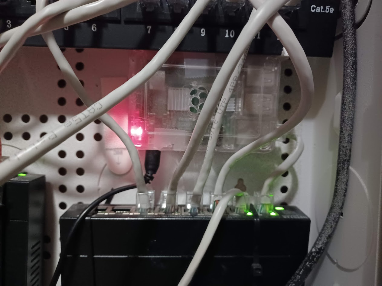
    Raspberry Pi connected to home network panel
    The Raspberry Pi, connected directly to the router. This is the server receiving and logging the temperature data.

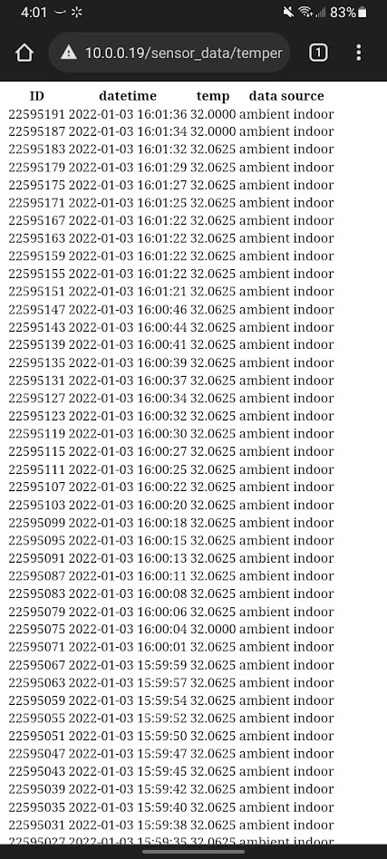
    I wrote a small web server so I could check temperatures from my phone. If someone was going to tell me the incubation temperature was wrong, I’d have a timestamped log at three-second resolution to discuss.

    Phone screen showing timestamped temperature log
    Raw temperature log. Timestamped, continuous, three-second resolution.

    Was this level of monitoring necessary for making tempeh? No. But the troubleshooting advice I kept getting was some variation of “your temperature was probably wrong,” and I was done guessing.

    The Wait

    After 12 hours: nothing visible. The bags looked exactly the same as when I loaded them.

    Four bags in incubator showing no visible change after twelve hours
    Twelve hours in. The bags look exactly the same.

    I wrote a pointed review of the tempeh starter on Amazon.

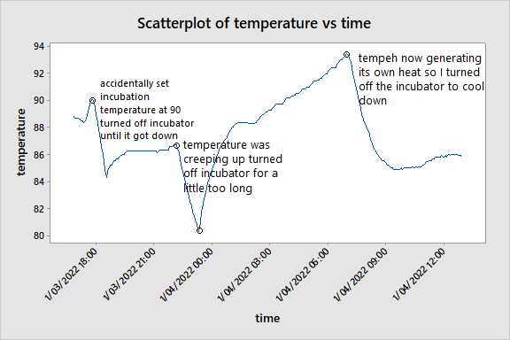
    But I checked back at lunch the next day and noticed something. The tempeh didn’t look different yet, but the temperature probe told a different story, the internal temperature was climbing above ambient. The beans were generating their own heat. Something was growing.

    Annotated scatter plot of temperature vs time
    The temperature log tells the whole story. You can see where I accidentally started at 90°F and had to let it cool, where the temperature crept up and I turned off the incubator a little too long, and finally, around hour 18, where the tempeh started generating its own metabolic heat. I turned the incubator off entirely and let the mold regulate itself.

    It Worked

    I opened the incubator and saw mycelium.

    White mycelium growing through the soybeans
    Mycelium. Finally.
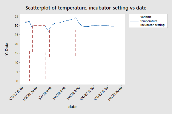
    Chart showing bean temperature vs incubator setting over time
    The full picture. Blue is the actual bean temperature; red dashed line is the incubator setting. At the end, the incubator is off and the tempeh is holding its own temperature around 30°C. Self-sustaining fermentation.

    A few more hours and the beans were fully bound together. Dense, white, solid blocks.

    Four completed blocks of tempeh
    Four blocks of finished tempeh. Uniform mycelium growth, firm structure.

    I changed my Amazon review.

    Amazon review updated to five stars
    “Pretty good. Don’t give up on it.” updated to 5 stars.

    What Actually Mattered

    The vague troubleshooting guides aren’t wrong, exactly. They’re just useless without measurement. “Too hot” and “too cold” don’t mean anything without a number attached. After going through this with three-second temperature resolution and documented steps, here’s what I think actually makes the difference:

    1. Dry the beans completely. Beyond “they look dry.” your hand shouldn’t feel any moisture when you grab a fistful. Then dry them a little more. Then add vinegar and dry that too.
    2. Start around 86°F (30°C), but watch it. Once the mold takes hold at around 18–24 hours, it generates enough metabolic heat to overshoot the optimal range. You may need to turn the incubator down or off entirely.
    3. Twelve hours of nothing is normal. The growth is invisible at first. If your temperature is in range and your beans were properly inoculated, wait. It happens fast once it starts.
    4. Measure what you can. You don’t need an ESP8266 and a Raspberry Pi (probably). But a probe thermometer inside the bean cake, rather than relying on the incubator’s ambient display, would have saved me several failed batches.

  • Hands-Free French Dictionary

    Hands-Free French Dictionary

    I have my concerns about AI coding.

    There’s an aphorism, the confidence about replacing a job with automation is highest when you are least familiar with it. For AI, in my domain, that’s been my experience. It can write SQL queries that run, but miss the context. It can scaffold out a Pytorch model, but in a tightly coupled overcommented mess. If you can one shot it, the code is great. Otherwise prepare for the slog.

    There’s a push and pull. You can see the rot happening when teams are pushed to use it entirely for development. I’m feeling the pressure to shoehorn it everywhere into my workflows. I’m left trying to protect future Jonathan on a Friday night. How can I use the 80% it can do well, but design a system that is efficient, and doesn’t sink the ship in the process. My systems won’t rot.

    Task

    I’m at the stage of learning French where I can read the newspaper or a novel, but not without stopping every couple of paragraphs to look something up. Solid B1, creeping toward B2. Every few lines there’s a word that could mean three different things depending on context, and if I just guess, I’m probably going to learn the wrong meaning and carry it around for months.

    The gold standard is looking it up and I have a 30-40 minute session daily where I look up words, write them down, do analytics later. The act of actively searching for a word builds stronger neural pathways than having someone hand you the answer. At the same time, you can’t use that approach 100% of the time. It’s cognitive strain maintaining it. When I’m reading on my couch, pick up my phone, open an app, type the word (with accents I don’t have memorized on the keyboard), read the definition, and then find my place again… I’m not reading anymore. I’m doing vocabulary drills that happen to be interrupted by a novel.

    I wanted something in between. Not a flashcard system, not a study tool. A way to keep reading without stopping too much, and without filling in the gaps wrong from context.

    Concept

    I started with a concept. I set my phone on the counter, or the table, or wherever I’m reading. When I hit a word I don’t know, I shout it out loud. The page would recognize the French, look up the definition, display it, and read it back to me. My eyes would never leave the page.

    It isn’t optimal for retention. I’m trading memory strength for reading flow. But the goal isn’t to memorize every word on first encounter. It’s to get through 40 pages instead of 12, and to not build a mental dictionary of wrong definitions by guessing from context clues that I’m not advanced enough to read correctly yet. Get to an hour of reading beyond the standard practice. The goal isn’t the new word to be learned, it’s reinforcing the other words as part of a sentence in new contexts.

    Webpage

    Straight across the plate. It would be a local app, single HTML file. I gave Claude a description of what I wanted and got back a 660-line HTML file that worked on the first run. Single file, no framework, no build step. It uses the built in Chrome voice recognition and an anonymous MyMemory translation API for French-to-English lookups, and in browser TTS to read it back. Simple.

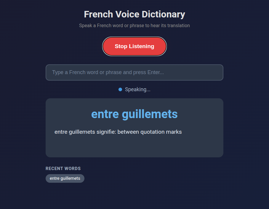
    French Voice Dictionary app showing the word entre guillemets with its translation between quotation marks, with a red Stop Listening button and dark themed UI
    Looking up “entre guillemets” (between quotation marks). Multi-word phrases work too.

    Phrases work too. “Entre guillemets” yields “between quotation marks.” That was a phrase that’s been rattling through my head because I hear it a lot on television (the news recently). Saying “dispositif de secours” gives me “backup device.” If I’m somewhere I can’t talk out loud, or the recognition is mangling my pronunciation on a specific word, there’s a text input as a fallback.

    The whole thing runs on GitHub Pages. No server, no cost, and I can pull it up on my phone’s browser while I read.

    Code Analysis

    The app worked, but some points crept up that I’ve seen when reviewing PRs at work too.

    Commenting

    Almost every block has a comment. // State above the state variables. // DOM Elements above the DOM queries. // Check browser support above the browser support check. // Timeout fallback in case onend never fires (browser quirk) above the timeout fallback. // Estimate ~100ms per character at 0.9 rate, plus 2 second buffer above the math that does exactly that.

    The system makes sense. The main issue with comments and documents is that it’s easy to make, impossible to maintain. If an LLM is able to make and update comments, and it helps as useful metadata for a downstream to read it, maybe it isn’t a problem. But in this instance, they describe what the next line does, not why. The kind of comments you’d delete in code review because the code already says it.

    State Flags

    The approach to concurrency was to add a boolean. Six flags at the top of the script: isListening, isProcessing, isSpeaking, pendingWord, lastProcessedWord, currentTTSTimeout. This is a three-state machine (listening, processing, speaking) implemented as a bag of independent booleans that have to be manually kept in sync. Every function checks two or three flags before deciding what to do. It works, but it’s the kind of thing where adding one more feature means touching every function.

    Tight Coupling and Separation of Concerns

    handleWord() updates the UI, manages API calls, state flags, interrupt detection, TTS triggering, and history. Six jobs. There’s no separation between “figure out the translation” and “update the screen” and “manage the audio pipeline.” If you wanted to swap the translation API, you’d be editing the middle of a 60-line function that also handles the queue logic. The code reads top to bottom like a script, and to its credit, the flow is clear. But it’s procedural, not structured.

    Though this one is counter to how I’ve normally seen its approach. When people code, I notice premature abstraction. Someone writes a data connector for a specific REST api, reasons they need to have one that actually should handle any number of internal APIs, or that it should be a general purpose data ingestion function, or more general purpose data provider function, … ultimately becoming a mess of overabstracted logic when a specific function would have fared better, even if there was theoretically some technical debt. AI usually flips this, making a bunch of concrete interconnected pieces that are nearly impossible to reason through. An AI can hold 15 objects in its mind while implementing a new change on a function, a human reviewer can’t.

    Broken Features

    Getting speech recognition to work was straightforward. Getting it to work continuously was a different story.

    The first version worked fine for one word. Say “bonjour,” get a definition, great. Say a second word and nothing happened. The app looked alive. The button still said “Stop Listening,” the status dot was green. No response.

    While the app processed a word (the API call, then the text-to-speech playback), a flag blocked all incoming speech. Anything I said during that window got dropped silently. No error, no feedback, just gone. And the browser’s text-to-speech onend event sometimes just doesn’t fire. Known quirk, no fix. When that happened, the flag stayed on forever and the app was bricked until I refreshed.

    It got worse before it got better. At one point the microphone was re-prompting for permission on every recognition cycle. The app started catching its own TTS output and trying to look up its own definitions in an infinite loop. We didn’t just screw the pooch. Basically every dog in the neighborhood.

    Problem Fixing Process

    I asked the AI to analyze the problem first, and it nailed the diagnosis: six potential causes, correctly prioritized, with the right recommendation (let speech interrupt TTS). Then I told it to implement the fix.

    It added three more state flags. lastRestartTime to throttle restarts. restartFailCount for exponential backoff. isStarting to prevent overlapping start attempts. The restart function went from 4 lines to 20, with timing checks, failure counters, and a “too many rapid restarts, stopping” error message. Net change: +41 lines.

    This made things worse. More flags meant more edge cases, more timing windows where flags disagreed, more ways for the state to get stuck. I spent a 22-message session debugging the debugging.

    The actual fix was the opposite: I deleted almost everything it had added. Removed all three new flags. Removed the backoff logic. Removed the duplicate word detection. The restart function went back to 4 lines. The real solution was simpler: stop the microphone during text-to-speech, restart it after. No timing, no counters, no tracking. The commit was -88 lines, +34 lines. The app ended up shorter than the initial generation despite having more functionality.

    Same pattern with gender detection. The AI built a suffix-matching heuristic for French noun gender (words ending in “-tion” are feminine, “-age” is masculine) and used it to prepend “un” or “une” to translation results. The badge in the UI? Fine, helpful visual hint. Prepending articles to verbs and adverbs? Not fine. I told it to remove the article logic entirely. A heuristic accurate enough for a colored dot is not accurate enough for constructing grammar.

    I tried adding English text-to-speech for the translation portion, so it would say “femme signifie” in French and then “woman” in English. Switching TTS languages mid-sentence didn’t work in any browser I tested. Killed it after one session.

    Overall Patterns

    Every correction I made was a deletion. The AI’s instinct, when something broke, was to add machinery. More flags, more tracking, more edge cases, ironically more brittleness. My instinct was to find the simpler fix that made the machinery unnecessary. At work I’ll often cherry pick/break up functions and use them, and sometimes the most sensible solution is to fail. It solved problems by building around them. I solved them by removing the complexity around them.

    The initial generation is often good. It gets me from concept to working app in one prompt, and the architecture is readable even if it was tightly coupled. But the debugging revealed that consistent bias. It writes like someone who’s read a lot of code but hasn’t maintained any of it. “Will this work” at the expense of “will this be easy to change later.” A human coder understands their limited capacity to hold things in their head. It drives simpler and more robust solutions. If an AI has a million token context window, why engineer anything that is less efficient? It can always figure it out later.

    For a side project I use on my couch while reading French novels, that’s completely fine. But if I were building something larger, I’d treat the output the way I’d treat a first draft as a way to challenge my initial approach. Sometimes the AI writes code in a way I’d never think of, but often in a way I should never think of. I’m working on understanding the 80% that works. The judo of redirecting the majority of the code into logical units that are easy to reason through and maintain.

    It’s a personal project. I can read my book without stopping. That has to count for something.

  • Training a Neural Net to Find Puss in Boots

    Training a Neural Net to Find Puss in Boots

    I want to fine-tune an image generation model on Puss in Boots. That means I need 50 to 100 good stills of the character. The movie is 98 minutes long. I am not going to sit there and screenshot by hand.

    So I trained a binary classifier to do it for me, wired it up to OBS, and let it watch the movie while I did other things. Here’s how that went.

    Step 1: Get some frames to label

    First problem, you need labeled data to train a classifier, but the whole point of the classifier is to avoid labeling by hand. Chicken McCrispy meet Egg McGriddle. I did a bootstrap, label a few images at first, and then strategically find new information. I started off by extracting 500 frames from the movie and manually putting them into puss/not-puss folders.

    def random_sample(video_path, output_dir, n=500, seed=42):
        random.seed(seed)
        cap, sar, fps, duration_sec = _video_info(video_path)
        timestamps = sorted(random.uniform(0, duration_sec) for _ in range(n))
    
        for ts in timestamps:
            cap.set(cv2.CAP_PROP_POS_MSEC, ts * 1000)
            ret, frame = cap.read()
            if not ret:
                continue
            frame = _correct_frame(frame, *sar)
            filename = f"frame_{ts:08.2f}s.jpg"
            cv2.imwrite(str(output_dir / filename), frame,
                        [cv2.IMWRITE_JPEG_QUALITY, 95])

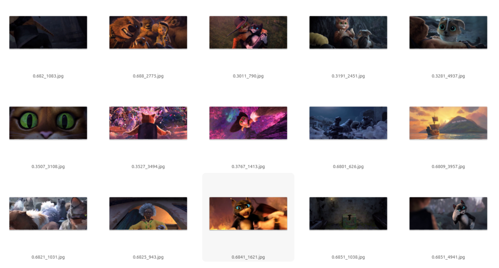
    After that, I trained the model (more on that below), then fetched 5000 more frames, and went back and looked at ones it got wrong with high confidence. If the model marked a new image of Puss in Boots at 95% confidence, then it has enough information. Marking a single shot of Perrito at 95%? That’s new information.

    File manager grid showing high-confidence false positives. Each filename starts with the classifier confidence score followed by a frame number.
    High-confidence false positives. Each filename starts with the model’s confidence score (e.g. 0.9872), followed by a frame number. These frames scored above 90% “puss” but contain no Puss in Boots: dark scenes, other characters, extreme close-ups of eyes. Good candidates for relabeling into the training set.

    I moved borderline cases and confident mistakes into the training folders and retrained. After a few rounds: 1,265 labeled frames total, 901 puss and 364 not-puss.

    Step 2: What the classifier has to learn

    This isn’t as simple as “find the orange cat.” The movie has other cat characters. Kitty Softpaws is also orange-ish and shows up in many of the same scenes. The classifier has to distinguish Puss specifically, across different lighting, angles, and scales (sometimes he’s a tiny figure in a wide shot, sometimes it’s an extreme close-up).

    Puss in Boots standing on a table with sword drawn, used as positive training example for the classifier

    puss = 1
    A nobleman character from the movie — clearly not Puss in Boots

    puss = 0

    Step 3: Training

    I went with ResNet18. Standard fine tuning workflow. Use a pretrained model, freeze most of it, unfreeze the last residual block and swap in a new classification head.

    ResNet(
      (conv1): Conv2d(3, 64, kernel_size=(7, 7), stride=(2, 2), padding=(3, 3), bias=False)
      (bn1): BatchNorm2d(64)
      (relu): ReLU(inplace=True)
      (maxpool): MaxPool2d(kernel_size=3, stride=2, padding=1)
      (layer1): Sequential(...)  # frozen
      (layer2): Sequential(...)  # frozen
      (layer3): Sequential(...)  # frozen
      (layer4): Sequential(       # unfrozen
        (0): BasicBlock(
          (conv1): Conv2d(256, 512, kernel_size=(3, 3), stride=(2, 2), padding=(1, 1))
          (bn1): BatchNorm2d(512)
          (conv2): Conv2d(512, 512, kernel_size=(3, 3), stride=(1, 1), padding=(1, 1))
          (bn2): BatchNorm2d(512)
        )
        (1): BasicBlock(...)
      )
      (avgpool): AdaptiveAvgPool2d(output_size=(1, 1))
      (fc): Linear(in_features=512, out_features=1, bias=True)  # replaced
    )

    One output neuron, BCEWithLogitsLoss, 15 epochs on CPU. I used weighted random sampling because my classes were imbalanced (more puss than not-puss, which, fair enough, he is the main character).

    model = models.resnet18(weights=models.ResNet18_Weights.DEFAULT)
    
    for name, param in model.named_parameters():
        if not name.startswith("layer4") and not name.startswith("fc"):
            param.requires_grad = False
    
    model.fc = nn.Linear(model.fc.in_features, 1)

    Out of 11.2 million parameters, 8.4 million were trainable. Validation accuracy hit 92.1% at best, but I was also going a little overboard with the complexity of the images it was using for tagging.

    Here’s what 92% looks like in practice. Both of these were labeled puss = 1 in the training set:

    Kitty Softpaws and Puss in Boots together in a fire scene

    puss = 1 (he’s in there, behind Kitty)
    Wide shot of a room with Puss in Boots barely visible at the left edge

    puss = 1 (hat visible at the left edge)

    The movie is 2.39:1 widescreen, but ResNet takes 224×224 square inputs. Every frame gets resized to fit that square, so widescreen shots get squeezed horizontally. In a wide shot where Puss is a small figure at the edge of the frame, he might occupy 20 pixels of the input tensor. The model still has to learn that counts. These borderline cases are part of why accuracy plateaus at 92% instead of 99, and also why 92% is fine for my purposes. The hard cases are genuinely hard.

    That’s not going to win any competitions, but I don’t need it to. I just need it to catch most frames of my dear Puss in Boots so I can sort through a smaller pile by hand instead of watching the whole movie frame by frame.

    Step 4: The source quality question

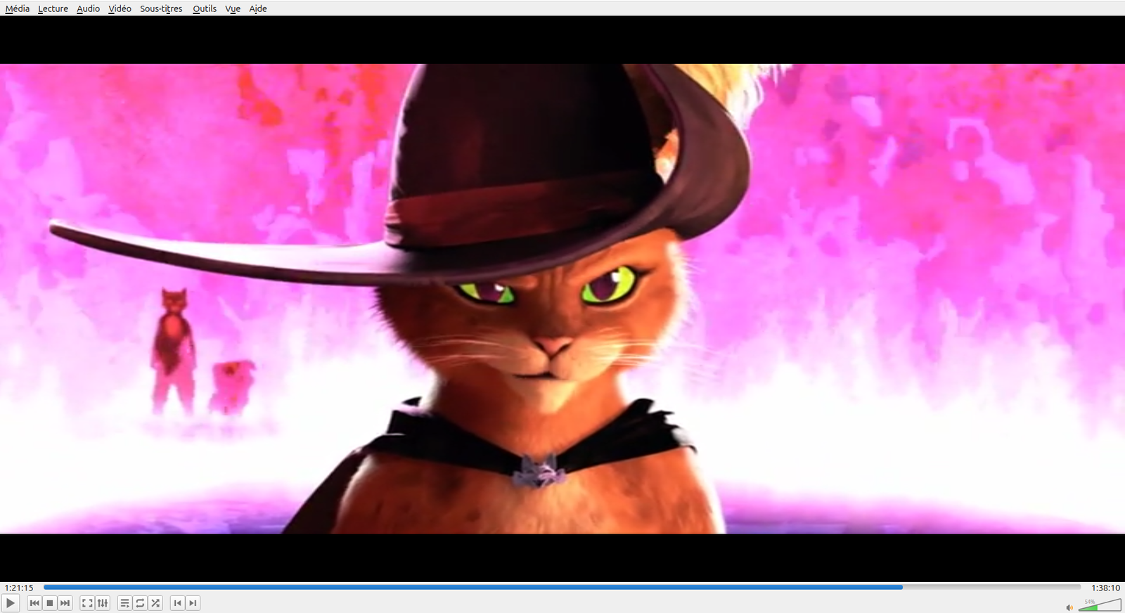
    Before building the live capture I got sidetracked wondering whether my video source was high enough quality for LoRA training. I spent a while comparing different copies and resolutions, checking codecs, obsessively alt-`ing between frame grabs. At one point I was pricing USB Blu-ray drives.

    Puss in Boots frame playing in a video player, used as source material for the frame extraction pipeline
    Frame grab from the source video. Good enough?

    Then I stopped and thought about it for a second. LoRA training data doesn’t need to be 4K. It needs variety: different poses, angles, lighting. A 98-minute movie has plenty of that regardless of resolution. I was solving the wrong problem.

    Step 5: Live capture

    This part I’m proud of. The beauty of PyTorch is that you can implement exotic logic and have something fundamentally editable. If you’re willing to relax these, you can get a much more performant model. Export the trained model to ONNX so you don’t need PyTorch at runtime, just onnxruntime and OpenCV. A future project I want to see how light a system I can get a useful ONNX model running.

    Open a Jupyter notebook. Point it at the OBS virtual camera. Every frame gets run through the model. Anything above 85% confidence gets saved to disk, with a one-second cooldown to avoid saving the same frame fifty times.

    cap = cv2.VideoCapture(VIDEO_SOURCE)
    
    while cap.isOpened():
        ret, frame = cap.read()
        if not ret:
            continue
    
        prob = predict(frame)
        now = time.time()
    
        if prob >= 0.85 and (now - last_save_time) >= 1.0:
            ts = datetime.now().strftime("%Y%m%d_%H%M%S_%f")
            filename = SAVE_DIR / f"puss_{ts}_{prob:.3f}.png"
            cv2.imwrite(str(filename), frame)
            last_save_time = now

    I added an overlay that shows up in the notebook cell: green text with the confidence percentage when Puss is on screen, red when he’s not. There’s a “[SAVED]” flash and a running count. So you can watch it work. Hit play in one window. Let the notebook chug in another. Go make coffee. Come back to 166 screenshots of a small orange cat in a hat.

    Puss in Boots standing with Kitty Softpaws and Perrito, captured by the classifier at 94.3% confidence
    The classifier handles group scenes. 94.3% with two other characters in frame.

    Results

    166 captures from one sitting. Confidence scores between 0.851 and 0.998. Most of them look good. The ones that don’t are motion blur: the classifier sees enough orange to think “that’s him” but the frame is a smear. Fair enough.

    A blurry frame with motion blur showing mostly furniture, incorrectly captured by the classifier at 86.1% confidence
    86.1% confidence. I think that’s a boot? The classifier is being generous.

    I ran perceptual hashing over the keepers to drop near-duplicates (distance threshold of 10), and ended up with about 70 distinct frames. That’s the LoRA dataset. Next I need to caption them and train the image model. But that’s a different project and a different post.

    Puss in Boots standing in the rain wearing his hat, captured automatically by the classifier with 97.6% confidence
    97.6% confidence. The hat helps.