Category: Machine Learning

Hands-on machine learning practice, from training runs to knowing when not to model.

  • When the Model Isn’t the Answer

    If you stare at any two datasets long enough, you can convince yourself there’s a connection between them. Not because there is, but because there is an important enough question that the data “should” be connected. It’s a dangerous place from which to start a modeling project.

    This is one such story. Enter multi-instance-learning, and how I failed spectacularly even on simulated data.

    Business Context

    Imagine an operation where some things are measured obsessively, but others are scattered. Precise timestamps on every step of a process. How long did each phase take? Detailed duration metrics on every transaction, high volumes every day.

    Separately, you run satisfaction surveys. Happy people interacting with your operation isn’t just a people thing. If you have a reputation for wasting someone’s time, you’re going to quickly find yourself paying more for the privilege. Making your operation a place people want to come is as good people sense as it is business.

    Not everyone takes the survey. It’s voluntary, and the responses come in throughout the day, timestamped but not tied to any specific transaction. Someone fills one in right after their interaction, and someone else two hours later, or the next morning. You don’t know which transaction prompted the response.

    In this scenario, we wouldn’t want to know what specific transaction prompted that response, and that isn’t important. We would like to know what conditions prompted it. If you found out that for whatever reason blue paint in the waiting room made people happy? Then blue paint it would be.

    The question I was wanting to answer: can we link those two data sources? If we could add contextual information to the survey, we could identify the operational metrics that actually matter to the people filling them out. Instead of guessing that long wait times hurt satisfaction, we’d have data. We could focus on the metrics that matter and surface them in operational dashboards, and have a balanced scorecard approach.

    I decided to throw a neural network at it. This is the story of why that was the wrong tool for the job.

    The Architecture

    The problem breaks down into two pieces you have to solve at once. You get a survey with a timestamp and a score, and somewhere in the hours before that survey, there’s a set of transactions that could have caused it. Which one was it? And what about that transaction made them rate it the way they did? You can’t answer one without the other. To learn what drives bad scores you need to know which transaction provoked it, but to know which transaction to look at you need to know what bad scores look like. Chicken and egg.

    I went at this two ways. First attempt was two networks trained together. One network looks at all the candidate transactions in a time window and assigns probability weights to each one, like saying “I think it was 60% likely to be transaction #47 and 25% likely to be transaction #52.” The other network takes a transaction’s duration metrics and tries to predict the survey score. They share a loss function, so when the score predictor gets it wrong, that error signal also teaches the matcher to pick better candidates next time.

    Second attempt used something called Multiple Instance Learning, where you treat all the candidate transactions as a bag. Instead of picking one candidate, the model weighs the whole set, builds a blended representation, and predicts the score from that. More mathematically principled for this kind of “I don’t know which item in the group is the important one” problem.

    Both are reasonable approaches. Neither was why things went sideways.

    The Synthetic Proof-of-Concept

    The exercise was built on proving out whether this could extract the signal from the noise when I knew there was a signal. I built a synthetic dataset with a known ground truth. 1,000 transactions, 200 surveys, a 30-minute candidate window. The scoring rule was deterministic: start at score 5, subtract points if any of four duration metrics exceeded their thresholds, floor at 1.

    Each survey was generated by randomly selecting a transaction and adding 2-30 minutes of delay. So I knew exactly which transaction caused each survey and I knew the exact formula that produced each score. No noise. No ambiguity. A few candidates per survey because the window was tight. If the model couldn’t crack this, it couldn’t crack anything.

    It got 85% of scores right and matched the correct transaction 80% of the time. Sounds decent until you remember this is a cheat sheet test. The formula is deterministic and there are maybe 4 candidates to pick from. Missing 15% of scores on that is not great. I looked at the training curves and it was classic overfitting. Train set accuracy going up, test set stuck and jittering around 75%. The model was fitting to the training examples rather than learning the pattern.
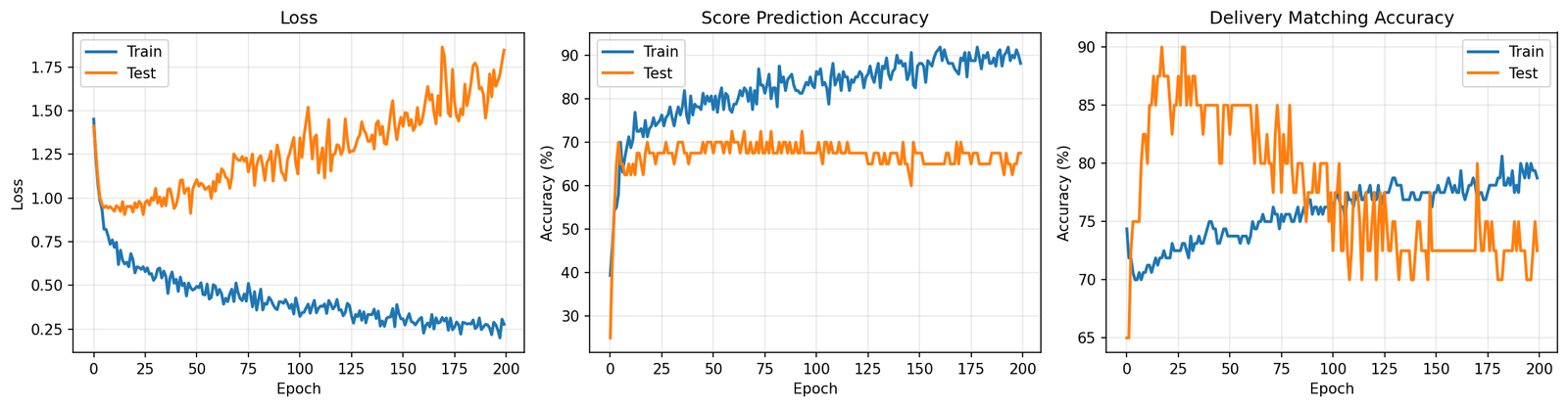
    Training curves showing loss, score prediction accuracy, and delivery matching accuracy over 200 epochs — train accuracy climbs to 90% while test plateaus around 75%, classic overfitting on synthetic data
    The synthetic version that actually learned something. The real data told a different story.

    That was the first red flag and I mostly ignored it.

    Scaling Up and Falling Apart

    I then tried to make the data look more like what you’d actually face in practice. Scaled to 10,000 transactions and 5,000 surveys. Widened the candidate window to 600 minutes. In practice, people don’t fill in surveys within 30 minutes. They do it hours later, sometimes the next day. A 600-minute window gave me about 40 candidates per survey instead of 4.

    Results: 35.9% score prediction accuracy, 2.7% transaction matching.

    Five score categories means guessing randomly gets you 20%. We barely beat random on scores. And 2.7% matching against 40 candidates is literally what you’d get from a coin flip (random chance is 2.5%). The model trained for 200 epochs and came out the other side knowing nothing it didn’t know before epoch 1.

    I switched to the MIL architecture. Loss went from 2.3 down to 1.6 over 65 epochs. Looks like progress on paper, but it’s a common trap: looking at loss functions and not considering what the model is actually doing with individual predictions. I pulled out the transactions the attention mechanism focused on most for each test survey and grouped them by score level.

    Score 1 transactions had average durations of 10.5, 7.6, 27.1. Score 5 transactions had average durations of 11.7, 7.5, 26.5. Basically the same numbers. The attention wasn’t locking onto anything meaningful. It picked whoever was convenient, and the score predictor just learned to always say “about 3.5” because that minimizes your loss when you have no real information.

    What I learned

    Three problems killed this, but any one of them would have sufficed.

    The Mechanical. The matching is looking for a needle in a haystack where all the hay looks exactly like the needle. Forty candidates in a window, all with duration metrics drawn from the same distributions. The correct transaction has no distinguishing mark. The only thing that makes it “correct” is that its durations happen to match the scoring formula, but the model doesn’t know the formula yet because that’s what it’s trying to learn. It’s stuck in a loop. You’d need something like a transaction ID on the survey, and if you had that, you wouldn’t need a model at all.

    The data collection. This one took me too long to see. A person filling out a survey isn’t reacting to one interaction. They’re reacting to their morning. Their week. How things have been going in general. The whole premise of “which transaction caused this score” assumes a 1-to-1 link that doesn’t exist. In practice, the extremes (1s and 5s) tend to reflect overall sentiment or first impressions, while the middle scores (2-4) are more nuanced. The survey is a thermometer, not a receipt.

    The business context. Even if you could match perfectly, a handful of duration numbers aren’t enough to explain why someone rates a 3 versus a 4. Experience depends on how people treated them, physical conditions, whether things were ready when they arrived, the weather. Duration is a proxy for some of that (long waits often signal a disorganized operation), but a rough one. Predicting 5-level satisfaction from timing features was always going to cap out.

    The Actual Answer

    The hypothesis behind all of this was something like: “if we reduce wait times, satisfaction goes up.” That’s a perfectly testable idea. But not with a model.

    Building a neural network to reverse-engineer causality from observational data is the hard way to answer this. The easy way: pick a set of locations, implement a change at half of them, leave the rest as controls, compare survey scores three months later. If cutting time moves the average score meaningfully, there’s your answer. The question becomes quantifying the value of that improvement and whether the cost pencils out. If it doesn’t budge, that’s also useful, and a lot cheaper than training models that converge to random, or worse relying on their recommendations.

    That’s the unglamorous conclusion. I spent time on attention mechanisms and MIL architectures when the right approach was a spreadsheet and a pilot program. I was trying to shortcut around the hard part (actually changing operations and measuring the result) by mining historical data for patterns that would predict the outcome. But the signal was never in the data because nobody designed the data collection to put it there. Surveys and transactions are two streams that happen to coexist in time. No amount of matrix multiplication will manufacture a causal link the measurement system never established.

    Sometimes you just have to run the experiment. Change the process and see what happens. No model required.

  • The Boring Part of Machine Learning Nobody Wants to Talk About

    The Boring Part of Machine Learning Nobody Wants to Talk About

    I’ve been getting more into vision analytics, private, professional, everywhere. My usual approach for solving problems is to learn a tool, understand conceptually what it does, check my back catalog of problems I couldn’t solve and see if that tool or approach helps. Vision analytics is no different.

    I’ve also applied this to document classification problems, imagine a thick scanned packet where you need to find specific data elements within specific pages among dozens of irrelevant ones. For the start, we trained a PyTorch model to filter out irrelevant pages in the packet based off how they “looked.” You don’t need to read the fine print to tell a calibration certificate from a cover sheet. I want to hone in on something we did for that project.

    A simple example, every ML tutorial skips the annotation step. You get “collect your data” and “train your model” with nothing in between. The in-between is where I’ve spent most of my time on this project. How do we really solve this problem?

    Off the shelf tools I’ve found include LabelImg for bounding box annotation with YOLO export, and Label Studio for more general-purpose labeling including classification. You can also save a bunch of files to a folder and manually drag things over, like I did for my Puss in Boots classifier. Each one of them requires you to learn a system that includes features not relevant for what you’re doing.

    For me, I knew the inputs (big folder of images), the outputs (the standard for YOLO and COCO are relatively clear). What was available to me? Touchscreen laptop, ways of interacting that I like, apps that I’ve liked using (e.g. I like bounding boxes you can click on to select, resize on the corners and not the outside of the box, being able to reclass by clicking the class again, …). What design choices work for me in the app are different than other people.

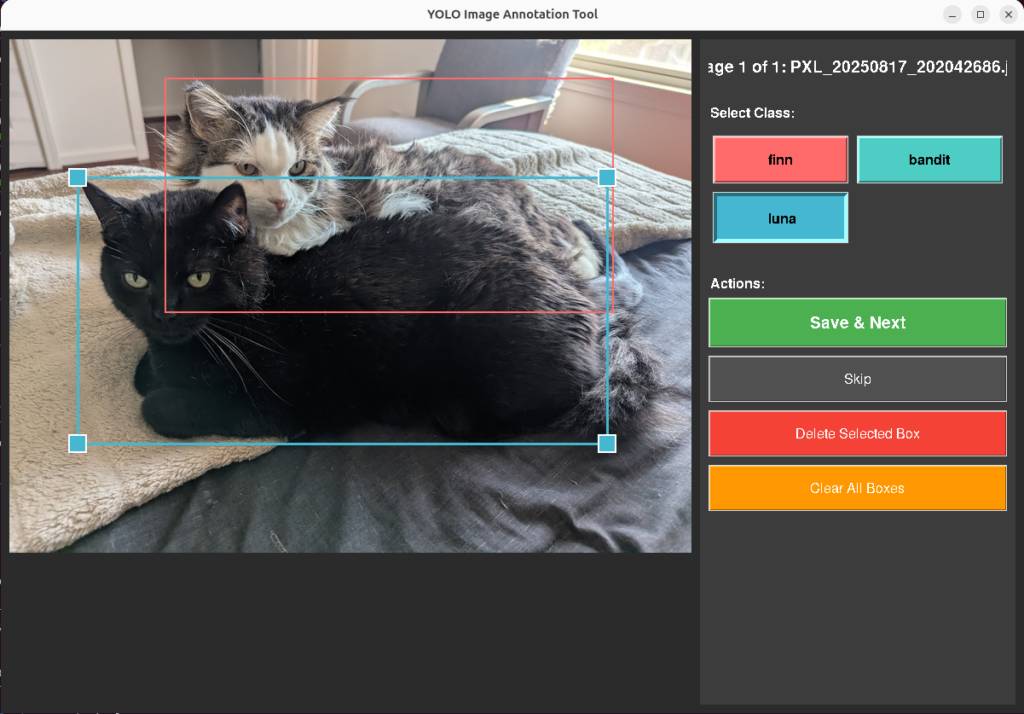
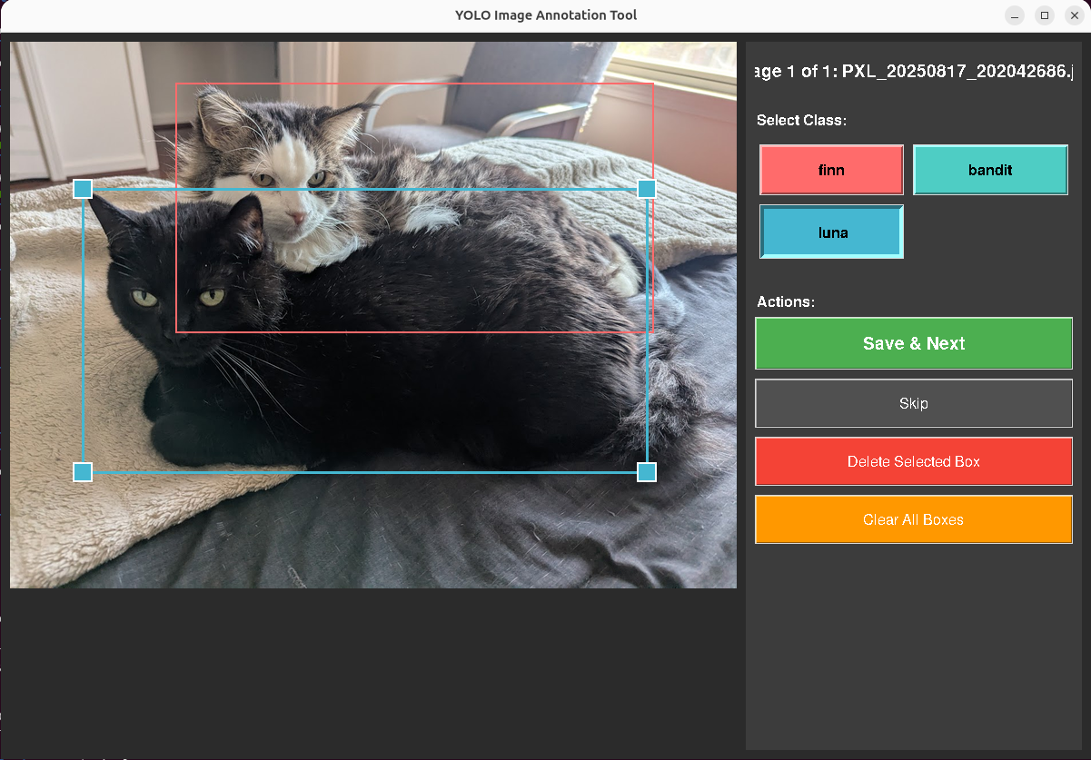
    With that, I built two versions of a bounding box annotation tool in tkinter. Both take images from an input directory, let you draw and label rectangles, and save bounding box coordinates in standard formats. The tool uses the touchscreen extensively, and the design choices you can see are all built for making that workflow simple, and simple for my brain.

    Screenshot of a tkinter-based YOLO annotation tool showing bounding boxes drawn around two cats, with class selection buttons and save controls on the right panel
    The first version of the annotation tool. Functional, if not pretty.

    Each annotation is a set of bounding box coordinates (class, position, size), one file per image. The tool manages file state: images go from data/input/ to data/processed/, annotations save to data/annotations/. An MD5 hash index checks each incoming image against already-processed files to prevent reannotating duplicates.

    Design Decisions

    These came from annotating about 200 images on a touchscreen tablet.

    Touch targets. Default tkinter handle sizes are too small for fingers. I set HANDLE_SIZE to 20 pixels, EDGE_TOLERANCE to 15, BUTTON_HEIGHT to 50. At the original sizes I was missing resize handles about 40% of the time on the touchscreen.

    Nested boxes. The cat detector needs both full-body and face annotations, meaning a smaller box inside a larger one. Click detection uses edge proximity: within EDGE_TOLERANCE pixels of an existing box edge means selection. Deeper inside means start drawing a new box. This solved the sub-annotation problem without adding a mode toggle.

    Auto-advance. Save and Next moves the image to processed/ and loads the next one. Saves roughly 4 seconds per image. Over 600 images, that’s 40 minutes of file management that the tool handles instead of me.

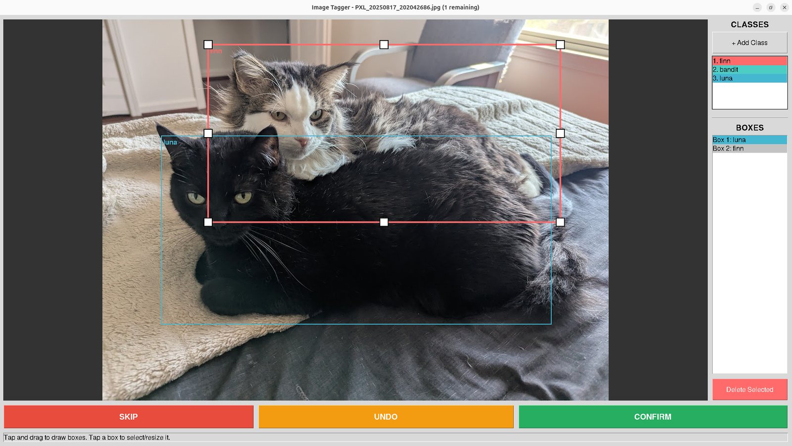
    Screenshot of the improved Image Tagger tool showing the same two cats with bounding boxes, featuring a class list panel, box inventory, and large SKIP/UNDO/CONFIRM buttons along the bottom
    Version two. Class panel, box inventory, and buttons you can actually hit with your fingers.

    V1 worked. V2 arose as I worked with the tool, noting every bit of hesitation I had with the interaction. I added undo/redo with a 50-action stack and a panel listing every box and its assigned class.

    From Cats to Documents

    For training images that just need a class label (like the original document classification problem), it’s still the same tool pattern, but in a different domain. I made another while thinking about how the project would work for documents. I in fact did this in the initial pass for the Puss in Boots detection, though at that scale, I started needing to be judicious about class balancing in the later rounds.

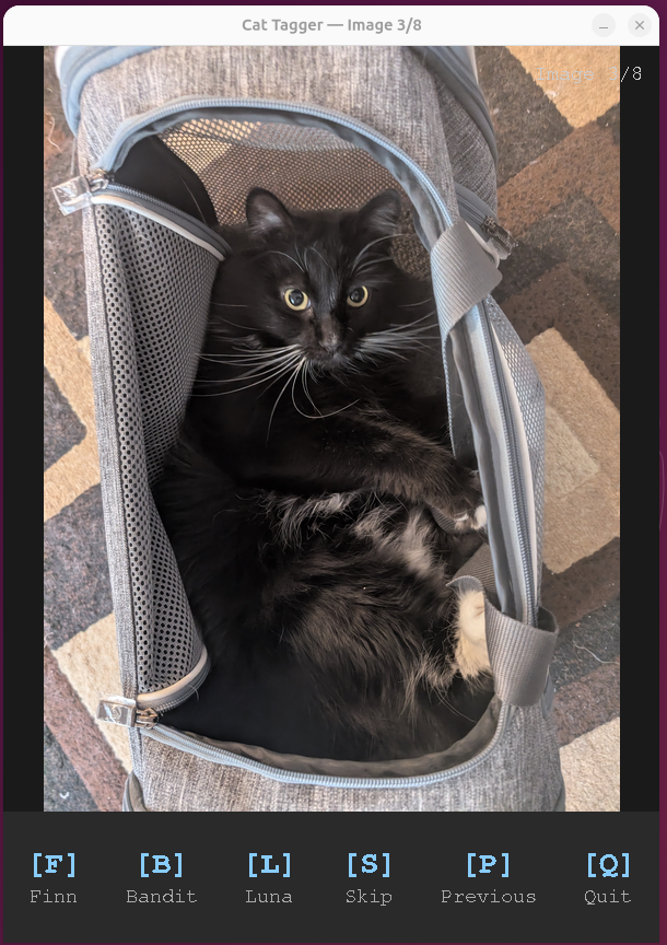
    For single image detection, keyboard tagging makes way more sense. I made a tool with Tkinter where it goes through the folder and displays it. You type F for Finn, B for Bandit, L for Luna. Same idea for documents: C for contract, I for invoice, R for receipt, S for skip. Image comes up, I press one key, next image loads. Peak throughput was about 1.5 seconds per page.

    Screenshot of a cat classification tagger tool showing two black cats in a crate, with keyboard shortcut overlay at the bottom: F for Finn, B for Bandit, L for Luna, S for Skip, P for Previous, Q for Quit
    Same pattern, different domain. Single-keystroke classification for cats.

    I’ve used the same pattern for document classification pipelines.

    What’s the point?

    I built these for myself not because that off-the-shelf tools can’t do classification. It’s that I can quickly and scrappily build something that identically matches how I’m already conceptualizing the process. Every shortcut, undo, go back, skip, exists because I hit that exact friction point while annotating. I add the stuff that makes it easy for me to do something extremely quickly, because the tool is just automating the way I’m already thinking about it. No translation costs accumulating.

    I don’t have to constantly think “okay, click, move the mouse to a point I wasn’t thinking about.” There’s no translation step between the decision in my head and the action the tool takes. That matters more than it sounds like it should. Ruts aren’t always a bad thing. Scale is easy to achieve if you’re working in them.

    A process that changes something, but closely enough to match the muscle memory of someone performing the task gets adopted. One that asks them to rethink their mental model on every interaction, doesn’t.

    End Result

    The tradeoff has always been between simple tools that work for most users (think things like coreutils in linux), more specialized powerful tools that work for an individual user (this post), and general purpose tools that work for everyone. The second two choices are becoming less of a distinction. Tkinter isn’t complex. It’s something that can be automated. Simple tools with reasoning and input a user can be glued together to make unreasonably powerful tools when paired with that user. The gap between “I need this tool” and “I have this tool” was two hours of tkinter and basic installs. That gap is getting smaller.

    Google’s been exploring an idea like this with Generative UI, where Gemini builds bespoke interfaces on the fly instead of showing everyone the same one. It’s the same process at a larger scale, since the question is built on “I need this output, but I want you to understand how it would be most straightforward for me to do it.”

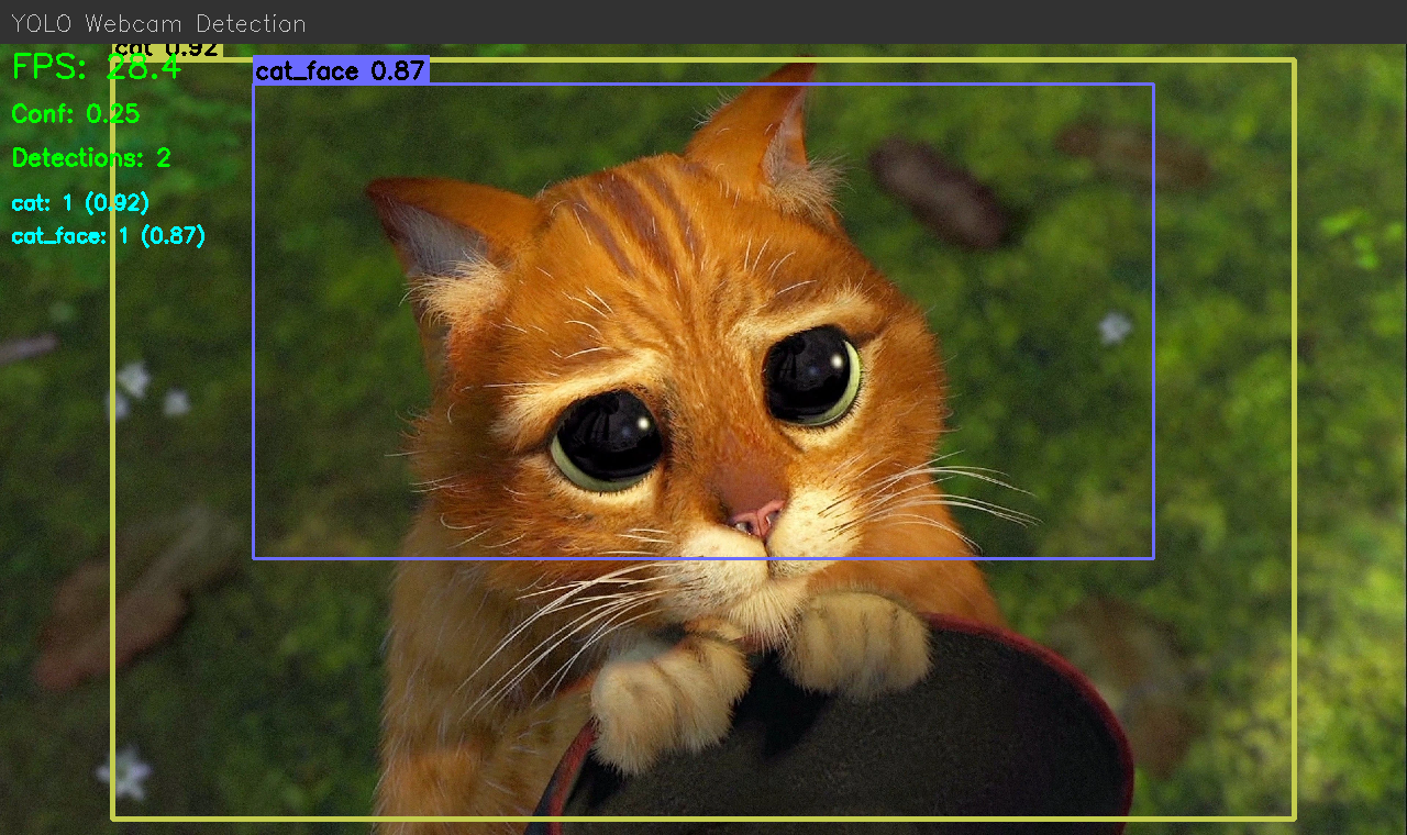
    YOLO webcam detection screenshot showing Puss in Boots with bounding boxes for cat (92% confidence) and cat_face (87% confidence), with FPS counter and detection stats overlay
    Annotated training data becomes a real-time detector.

    Ultimately, the tools I built here aren’t polished. They’re precisely fit. They’re held together with tkinter and duct tape, but that’s the point, built on the fly to match the shape of how I already think about the problem, so there’s no tax on every interaction. And that’s the real lesson here. The next generation of tooling isn’t going to be about building one perfect interface. It’ll be about making it trivially cheap to build the right interface for the person sitting in front of it.

  • Training a Neural Net to Find Puss in Boots

    Training a Neural Net to Find Puss in Boots

    I want to fine-tune an image generation model on Puss in Boots. That means I need 50 to 100 good stills of the character. The movie is 98 minutes long. I am not going to sit there and screenshot by hand.

    So I trained a binary classifier to do it for me, wired it up to OBS, and let it watch the movie while I did other things. Here’s how that went.

    Step 1: Get some frames to label

    First problem, you need labeled data to train a classifier, but the whole point of the classifier is to avoid labeling by hand. Chicken McCrispy meet Egg McGriddle. I did a bootstrap, label a few images at first, and then strategically find new information. I started off by extracting 500 frames from the movie and manually putting them into puss/not-puss folders.

    def random_sample(video_path, output_dir, n=500, seed=42):
        random.seed(seed)
        cap, sar, fps, duration_sec = _video_info(video_path)
        timestamps = sorted(random.uniform(0, duration_sec) for _ in range(n))
    
        for ts in timestamps:
            cap.set(cv2.CAP_PROP_POS_MSEC, ts * 1000)
            ret, frame = cap.read()
            if not ret:
                continue
            frame = _correct_frame(frame, *sar)
            filename = f"frame_{ts:08.2f}s.jpg"
            cv2.imwrite(str(output_dir / filename), frame,
                        [cv2.IMWRITE_JPEG_QUALITY, 95])

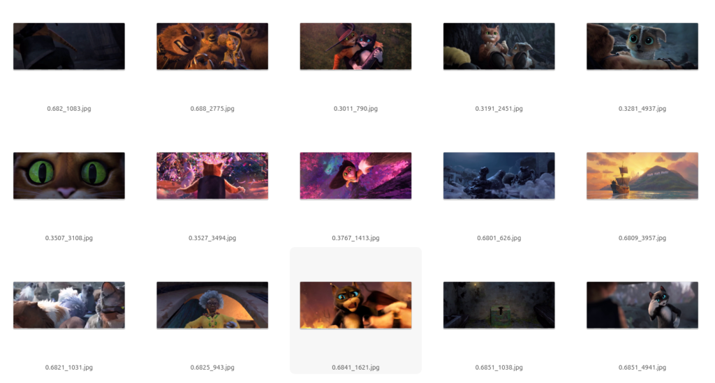
    After that, I trained the model (more on that below), then fetched 5000 more frames, and went back and looked at ones it got wrong with high confidence. If the model marked a new image of Puss in Boots at 95% confidence, then it has enough information. Marking a single shot of Perrito at 95%? That’s new information.

    File manager grid showing high-confidence false positives. Each filename starts with the classifier confidence score followed by a frame number.
    High-confidence false positives. Each filename starts with the model’s confidence score (e.g. 0.9872), followed by a frame number. These frames scored above 90% “puss” but contain no Puss in Boots: dark scenes, other characters, extreme close-ups of eyes. Good candidates for relabeling into the training set.

    I moved borderline cases and confident mistakes into the training folders and retrained. After a few rounds: 1,265 labeled frames total, 901 puss and 364 not-puss.

    Step 2: What the classifier has to learn

    This isn’t as simple as “find the orange cat.” The movie has other cat characters. Kitty Softpaws is also orange-ish and shows up in many of the same scenes. The classifier has to distinguish Puss specifically, across different lighting, angles, and scales (sometimes he’s a tiny figure in a wide shot, sometimes it’s an extreme close-up).

    Puss in Boots standing on a table with sword drawn, used as positive training example for the classifier

    puss = 1
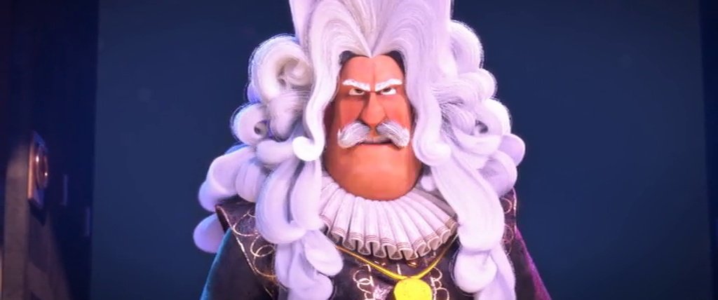
    A nobleman character from the movie — clearly not Puss in Boots

    puss = 0

    Step 3: Training

    I went with ResNet18. Standard fine tuning workflow. Use a pretrained model, freeze most of it, unfreeze the last residual block and swap in a new classification head.

    ResNet(
      (conv1): Conv2d(3, 64, kernel_size=(7, 7), stride=(2, 2), padding=(3, 3), bias=False)
      (bn1): BatchNorm2d(64)
      (relu): ReLU(inplace=True)
      (maxpool): MaxPool2d(kernel_size=3, stride=2, padding=1)
      (layer1): Sequential(...)  # frozen
      (layer2): Sequential(...)  # frozen
      (layer3): Sequential(...)  # frozen
      (layer4): Sequential(       # unfrozen
        (0): BasicBlock(
          (conv1): Conv2d(256, 512, kernel_size=(3, 3), stride=(2, 2), padding=(1, 1))
          (bn1): BatchNorm2d(512)
          (conv2): Conv2d(512, 512, kernel_size=(3, 3), stride=(1, 1), padding=(1, 1))
          (bn2): BatchNorm2d(512)
        )
        (1): BasicBlock(...)
      )
      (avgpool): AdaptiveAvgPool2d(output_size=(1, 1))
      (fc): Linear(in_features=512, out_features=1, bias=True)  # replaced
    )

    One output neuron, BCEWithLogitsLoss, 15 epochs on CPU. I used weighted random sampling because my classes were imbalanced (more puss than not-puss, which, fair enough, he is the main character).

    model = models.resnet18(weights=models.ResNet18_Weights.DEFAULT)
    
    for name, param in model.named_parameters():
        if not name.startswith("layer4") and not name.startswith("fc"):
            param.requires_grad = False
    
    model.fc = nn.Linear(model.fc.in_features, 1)

    Out of 11.2 million parameters, 8.4 million were trainable. Validation accuracy hit 92.1% at best, but I was also going a little overboard with the complexity of the images it was using for tagging.

    Here’s what 92% looks like in practice. Both of these were labeled puss = 1 in the training set:

    Kitty Softpaws and Puss in Boots together in a fire scene

    puss = 1 (he’s in there, behind Kitty)
    Wide shot of a room with Puss in Boots barely visible at the left edge

    puss = 1 (hat visible at the left edge)

    The movie is 2.39:1 widescreen, but ResNet takes 224×224 square inputs. Every frame gets resized to fit that square, so widescreen shots get squeezed horizontally. In a wide shot where Puss is a small figure at the edge of the frame, he might occupy 20 pixels of the input tensor. The model still has to learn that counts. These borderline cases are part of why accuracy plateaus at 92% instead of 99, and also why 92% is fine for my purposes. The hard cases are genuinely hard.

    That’s not going to win any competitions, but I don’t need it to. I just need it to catch most frames of my dear Puss in Boots so I can sort through a smaller pile by hand instead of watching the whole movie frame by frame.

    Step 4: The source quality question

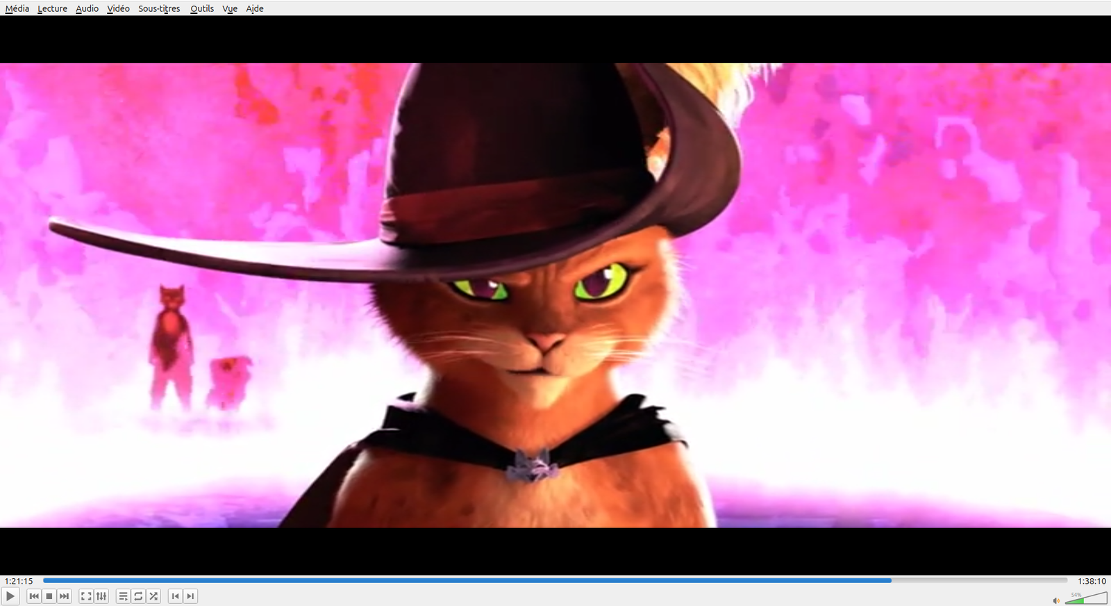
    Before building the live capture I got sidetracked wondering whether my video source was high enough quality for LoRA training. I spent a while comparing different copies and resolutions, checking codecs, obsessively alt-`ing between frame grabs. At one point I was pricing USB Blu-ray drives.

    Puss in Boots frame playing in a video player, used as source material for the frame extraction pipeline
    Frame grab from the source video. Good enough?

    Then I stopped and thought about it for a second. LoRA training data doesn’t need to be 4K. It needs variety: different poses, angles, lighting. A 98-minute movie has plenty of that regardless of resolution. I was solving the wrong problem.

    Step 5: Live capture

    This part I’m proud of. The beauty of PyTorch is that you can implement exotic logic and have something fundamentally editable. If you’re willing to relax these, you can get a much more performant model. Export the trained model to ONNX so you don’t need PyTorch at runtime, just onnxruntime and OpenCV. A future project I want to see how light a system I can get a useful ONNX model running.

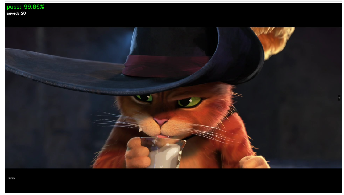
    Open a Jupyter notebook. Point it at the OBS virtual camera. Every frame gets run through the model. Anything above 85% confidence gets saved to disk, with a one-second cooldown to avoid saving the same frame fifty times.

    cap = cv2.VideoCapture(VIDEO_SOURCE)
    
    while cap.isOpened():
        ret, frame = cap.read()
        if not ret:
            continue
    
        prob = predict(frame)
        now = time.time()
    
        if prob >= 0.85 and (now - last_save_time) >= 1.0:
            ts = datetime.now().strftime("%Y%m%d_%H%M%S_%f")
            filename = SAVE_DIR / f"puss_{ts}_{prob:.3f}.png"
            cv2.imwrite(str(filename), frame)
            last_save_time = now

    I added an overlay that shows up in the notebook cell: green text with the confidence percentage when Puss is on screen, red when he’s not. There’s a “[SAVED]” flash and a running count. So you can watch it work. Hit play in one window. Let the notebook chug in another. Go make coffee. Come back to 166 screenshots of a small orange cat in a hat.

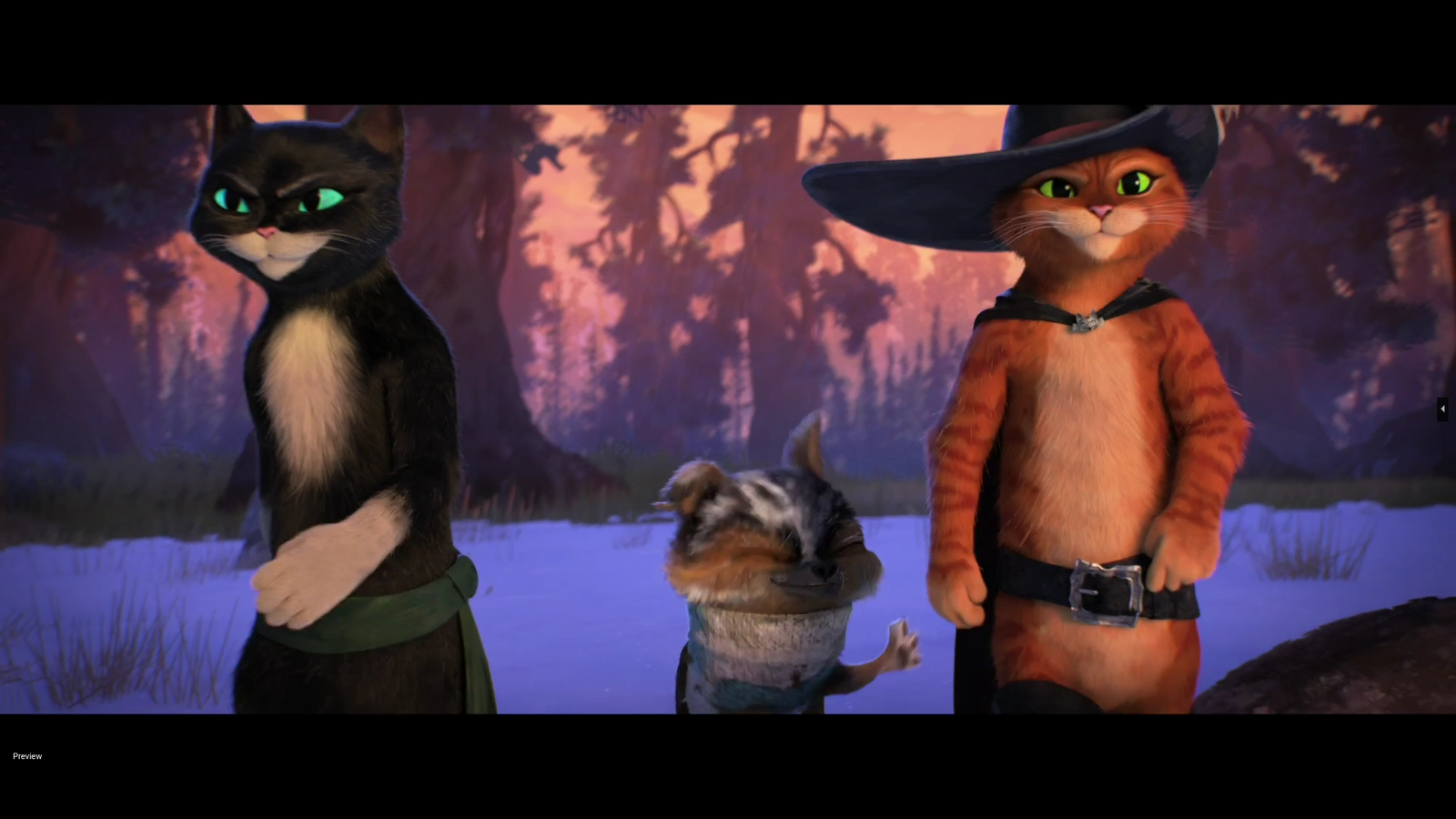
    Puss in Boots standing with Kitty Softpaws and Perrito, captured by the classifier at 94.3% confidence
    The classifier handles group scenes. 94.3% with two other characters in frame.

    Results

    166 captures from one sitting. Confidence scores between 0.851 and 0.998. Most of them look good. The ones that don’t are motion blur: the classifier sees enough orange to think “that’s him” but the frame is a smear. Fair enough.

    A blurry frame with motion blur showing mostly furniture, incorrectly captured by the classifier at 86.1% confidence
    86.1% confidence. I think that’s a boot? The classifier is being generous.

    I ran perceptual hashing over the keepers to drop near-duplicates (distance threshold of 10), and ended up with about 70 distinct frames. That’s the LoRA dataset. Next I need to caption them and train the image model. But that’s a different project and a different post.

    Puss in Boots standing in the rain wearing his hat, captured automatically by the classifier with 97.6% confidence
    97.6% confidence. The hat helps.